BPR

BPR 算法

显式反馈：用户对物品的评分，如电影评分；隐式反馈：用户对物品的交互行为，如浏览，购买等，现实中绝大部分数据属于隐式反馈，可以从日志中获取。BPR是基于用户的隐式反馈，为用户提供物品的推荐，并且是直接对排序进行优化。贝叶斯个性化排序（Bayesian personalized ranking，BPR）是一种 Pairwise 方法，并且借鉴了矩阵分解的思路。在开始深入讲解原理之前我们先了解整个 BPR 的基础假设以及基本设定。
因为是基于贝叶斯的 Pairwise 方法，BPR 有两个基本假设：

• 每个用户之间的偏好行为相互独立，即用户 u 在商品 i 和 j 之间的偏好和其他用户无关。
• 同一用户对不同物品的偏序相互独立，也就是用户 u 在商品 i 和 j 之间的偏好和其他的商品无关。

这里补充一下Pairwise。配对法(Pairwise)的基本思路是对样本进行两两比较，构建偏序文档对，从比较中学习排序，因为对于一个查询关键字来说，最重要的其实不是针对某一个文档的相关性是否估计得准确，而是要能够正确估计一组文档之间的 “相对关系”。
因此，Pairwise 的训练集样本从每一个 “关键字文档对” 变成了 “关键字文档文档配对”。也就是说，每一个数据样本其实是一个比较关系，当前一个文档比后一个文档相关排序更靠前的话，就是正例，否则便是负例，如下图。试想，有三个文档：A、B 和 C。完美的排序是 “B>C>A”。我们希望通过学习两两关系 “B>C”、“B>A” 和 “C>A” 来重构 “B>C>A”。

BPR 用来解决隐式反馈的推荐排序问题，假设有用户集 U 和物品集 I，当用户 u（u∈U）在物品展示页面点击了物品 i（i∈I）却没有点击同样曝光在展示页面的物品 j（j∈I），则说明对于物品 i 和物品 j，用户 u 可能更加偏好物品 i，用 Pairwise 的思想则是物品 i 的排序要比物品 j 的排序更靠前，这个偏序关系可以写成一个三元组 <u,i,j>，为了简化表述，我们用 >u 符号表示用户 u 的偏好，<u,i,j> 可以表示为：i>uj。单独用 >u 代表用户 u 对应的所有商品中两两偏序关系，可知 >u⊂$I^{2}$.
记 S 为所有用户对所有物品发生的隐式反馈集合，这里针对隐式反馈问题对评分矩阵进行了简化，即点击过则视为正例，记为 1；没点击过则视为负例，通常会置为 0，如下图所示：
.
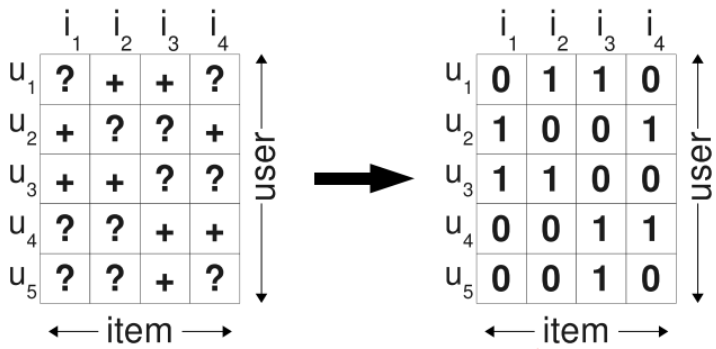BPR 试图通过用户的反馈矩阵 S 来为每一个用户构建出完整的偏序关系，也称全序关系，用 >u 表示.如下图所示：

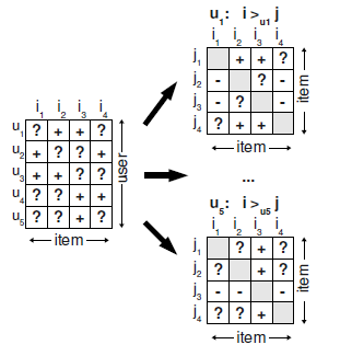
图左边的矩阵是反馈数据集 S，“+” 代表有反馈数据，“?” 代表无反馈数据。

图右边的小矩阵是每个用户的偏序关系矩阵，“+” 代表用户喜欢 i 胜过喜欢 j，作为训练数据的正例；“-” 代表用户喜欢 j 胜过喜欢 i，作为训练数据的负例；“?” 代表同类数据无法确定偏序关系。

比如用户 u1 看过产品 i2 但是没看过产品 i1，所以我们假设用户喜欢产品 i2 胜过 i1：即 i2>ui1。对于用户均产生反馈过的产品，我们不能推断出任何偏好，同样，对于那些用户都没有反馈过的两个产品，我们也不能推断出任何偏好。也就是说，两个有反馈数据之间以及两个无反馈数据之间都无法构建偏序关系。

为了形式化描述这种情形，我们定义训练数据 DS:U×I×I ：

$$D_{s}:=\{(u,i,j) | i \in I^{+}_{U} \bigwedge j \in I / I^{+}_{U} \}$$

其中 (u,i,j)∈DS 的表示是用户 u 更喜欢 i 胜过 j；∧ 是离散数学中的符号，表示 and，等同于 ∩；$I/I^{+}_{U}$ 表示物品集 I 除正例外其他剩余的样本。

BPR 模型本质是一种矩阵分解算法，所以其模型本质上是为了将用户物品矩阵分解成两个低维矩阵(用户矩阵($U*K$)和物品矩阵($I*K$))，在由两个低维矩阵相乘后得到完整的矩阵。即

$$\hat{x}=WH^{T}$$

对于任意一个用户u，对应任意一个物品i我们期望有：

$${\hat{x}}{ui}=w_{u}*h_{u}=\sum_{f=1}^{k}w_{uf}h_{if}$$

我们的目的就是找到合适的矩阵W,H让$\hat{x}$和X最相似。

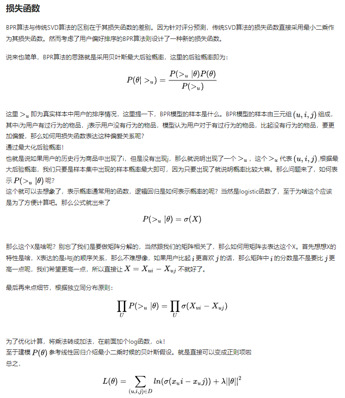
BPR损失函数

BPR 基于最大后验估计P(W,H|>u)来求解模型参数W,H,这里我们用θ来表示参数W和H, >u代表用户u对应的所有商品的全序关系,则优化目标是P(θ|>u)。根据贝叶斯公式，我们有：

$$P(θ|>u)=\frac{P(>u|θ)P(θ)}{P(>u)}$$

由于我们假设了用户的排序和其他用户无关，那么对于任意一个用户u来说，P(>u)对所有的物品一样，所以有：

$$P(θ|>u)∝P(>u|θ)P(θ)$$

这个优化目标转化为两部分。第一部分和样本数据集D有关，第二部分和样本数据集D无关。

对于第一部分，由于我们假设每个用户之间的偏好行为相互独立，同一用户对不同物品的偏序相互独立，所以有：

$$\prod_{u \in U}P(>_u|\theta) = \prod_{(u,i,j) \in (U \times I \times I)}P(i >_u j|\theta)^{\delta((u,i,j) \in D)}(1-P(i >_u j|\theta))^{\delta((u,j,i) \not\in D) }$$

其中，

$$\delta(b)= \begin{cases} 1& {if\; b\; is \;true}\\ 0& {else} \end{cases}$$

根据上面讲到的完整性和反对称性，优化目标的第一部分可以简化为：

$$\prod_{u \in U}P(>_u|\theta) = \prod_{(u,i,j) \in D}P(i >_u j|\theta)$$

而对于$P(i >_u j|\theta)$这个概率，我们可以使用下面这个式子来代替:

$$P(i >_u j|\theta) = \sigma(\hat{x}_{uij}(\theta))$$

对于$\hat{x}_{uij}(\theta)$，我们要满足当$i>_u j$时,$\hat{x}_{uij}(\theta)>0$,当$i<_u j$时,$\hat{x}_{uij}(\theta)<0$,所以有

$$\hat{x}_{uij}=\hat{x}_{ui}-\hat{x}_{uj}$$

最终，我们的第一部分优化目标转化为：

$$\prod_{u \in U}P(>_u|\theta) = \prod_{(u,i,j) \in D} \sigma(\hat{x}_{ui} - \hat{x}_{uj})$$

对于第二部分P(θ)，原作者大胆使用了贝叶斯假设，即这个概率分布符合正太分布，且对应的均值是0，协方差矩阵是$\lambda_{\theta}I$,即

$$P(\theta) \sim N(0, \lambda_{\theta}I)$$

对于上面假设的这个多维正态分布，其对数和$||\theta||^{2}$成正比。即

$$lnP(\theta) = \lambda||\theta||^2$$

最终对于我们的最大对数后验估计函数

$$ln\;P(\theta|>_u) \propto ln\;P(>_u|\theta)P(\theta) = ln\;\prod\limits_{(u,i,j) \in D} \sigma(\hat{x}_{ui} - \hat{x}_{uj}) + ln P(\theta) = \sum\limits_{(u,i,j) \in D}ln\sigma(\hat{x}_{ui} - \hat{x}_{uj}) + \lambda||\theta||^2\;$$

这里给出另外一种推导方法：原博客地址

接着使用梯度下降法来优化参数模型即可。

$$L(\theta)= \sum\limits_{(u,i,j) \in D}ln\sigma(\hat{x}_{ui} - \hat{x}_{uj}) + \lambda||\theta||^2\;$$

$$=\sum\limits_{(u,i,j) \in D}ln\sigma(w_{u}^{T} H_{i} - w_{u}^{T}H_{j}) + \lambda||\theta||^2\;$$

由于

$$ln(x)^{'}=\frac{1}{x}$$

$$\sigma(x)^{'}=\sigma(x)(1-\sigma(x))$$

$$(ln \sigma(x))^{'}=\frac{1}{\sigma(x)}\sigma(x)(1-\sigma(x))=1-\sigma(x)=1-\frac{1}{1+e^{-x}}=\frac{1}{1+e^{x}}$$

所以

$$\frac{\partial(L(\theta))}{\partial w_{u}}=\frac{1}{1+e^{x_{ui}-x_{uj}}}(H_{i}-H_{j})+\lambda w_{u}$$

$$\frac{\partial(L(\theta))}{\partial H_{i}}=\frac{1}{1+e^{x_{ui}-x_{uj}}}w_{u}+\lambda H_{i}$$

$$\frac{\partial(L(\theta))}{\partial H_{j}}=\frac{1}{1+e^{x_{ui}-x_{uj}}}(-w_{u})+\lambda H_{j}$$

Pytorch 实现

#####导包

import numpy as np
import pandas as pd
import scipy.sparse as sp
import torch.utils.data as data
import torch
import torch.nn as nn
import os
import time

数据处理

此数据集中UserID 0~4039 MovieID 0~3075
train.rating中一共994169行
train_mat (6040,3706)
test_data 604000

dataset = 'ml-1m'
main_path = './Data/'
train_rating = main_path + '{}.train.rating'.format(dataset)
test_rating = main_path + '{}.test.rating'.format(dataset)
test_negative = main_path + '{}.test.negative'.format(dataset)
model_path = './models/'
BPR_model_path = model_path + 'BPR.pth'

# 1、训练集
train_data = pd.read_csv(train_rating, sep='\t', header=None, names=['user', 'item'], 
    usecols=[0, 1], dtype={0: np.int32, 1: np.int32})
print(train_data)
user_num = train_data['user'].max() + 1
item_num = train_data['item'].max() + 1
print(train_data['user'].max())
print(user_num,item_num)
train_data = train_data.values.tolist()

        user  item
0          0    32
1          0    34
2          0     4
3          0    35
4          0    30
...      ...   ...
994164  6039  1092
994165  6039    41
994166  6039   128
994167  6039   323
994168  6039   669

[994169 rows x 2 columns]
6039
6040 3706

train_data1 = pd.read_csv(train_rating, sep='\t', header=None, names=['user', 'item'], 
    usecols=[0, 1], dtype={0: np.int32, 1: np.int32})

index=train_data1[(train_data1.user==745)&(train_data1['item']==510)].index.tolist()
train_data1.loc[index,:]

	user	item
114281	745	510

(train_data[:10])

[[0, 32],
 [0, 34],
 [0, 4],
 [0, 35],
 [0, 30],
 [0, 29],
 [0, 33],
 [0, 40],
 [0, 10],
 [0, 16]]

# 2、训练样本转换为稀疏矩阵
train_mat = sp.dok_matrix((user_num, item_num), dtype=np.float32)
for x in train_data:
    train_mat[x[0], x[1]] = 1.0

#print(train_mat)
train_mat
#train_data  994169行 记录用户给打过分的电影 如第一行 [0,34]代表第0个用户给地34部电影打过分
#train_mat 为稀疏矩阵，6040(用户)*3706(电影)
#            用户打过分的记为1否则为0
#test_data  604000 m每个用户一百个数据，一个打过分，99个没有打过分
# #

<6040x3706 sparse matrix of type '<class 'numpy.float32'>'
	with 994169 stored elements in Dictionary Of Keys format>

# 3、测试集数据读取,即为每个用户赋值99个没评分过的item。 1个评分过的+99个未评分的。
test_data = []
with open(test_negative, 'r') as fd:
    line = fd.readline()
    while line != None and line != '':
        arr = line.split('\t')
        u = eval(arr[0])[0]
        test_data.append([u, eval(arr[0])[1]])
        for i in arr[1:]:
            test_data.append([u, int(i)])
        line = fd.readline()

test_data

# 根据继承pytorch的Dataset类定义BPR数据类
class BPRData(data.Dataset):
    def __init__(self, features,
                 num_item, train_mat=None, num_ng=0, is_training=None):
        """features=train_data,num_item=item_num,train_mat，稀疏矩阵，num_ng,训练阶段默认为4，即采样4-1个负样本对应一个评分过的
        数据。
        """
        super(BPRData, self).__init__()
        """ Note that the labels are only useful when training, we thus 
            add them in the ng_sample() function.
        """
        self.features = features
        self.num_item = num_item
        self.train_mat = train_mat
        self.num_ng = num_ng
        self.is_training = is_training

    def ng_sample(self):
        assert self.is_training, 'no need to sampling when testing'

        self.features_fill = []
        for x in self.features:
            u, i = x[0], x[1]
            for t in range(self.num_ng):
                j = np.random.randint(self.num_item)
                while (u, j) in self.train_mat:
                    j = np.random.randint(self.num_item)
                self.features_fill.append([u, i, j])

    def __len__(self):
        return self.num_ng * len(self.features) if \
            self.is_training else len(self.features)

    def __getitem__(self, idx):
        features = self.features_fill if \
            self.is_training else self.features

        user = features[idx][0]
        item_i = features[idx][1]
        item_j = features[idx][2] if \
            self.is_training else features[idx][1]
        return user, item_i, item_j

#生产datalodaer
train_dataset = BPRData(
        train_data, item_num, train_mat, 4, True)
test_dataset = BPRData(
        test_data, item_num, train_mat, 0, False)
train_loader = data.DataLoader(train_dataset,
                                   batch_size=4096, shuffle=True, num_workers=0)
test_loader = data.DataLoader(test_dataset,
                                  batch_size=100, shuffle=False, num_workers=0)

train_loader.dataset.ng_sample()
for x,y,z in train_loader:
    print(x,y,z)
    break

tensor([2276, 4534, 2665,  ..., 5975,  720, 5452]) tensor([ 733,  385,  517,  ...,  714, 2270,   60]) tensor([ 800, 2328,  641,  ..., 3351, 2708, 3218])

x.shape

torch.Size([4096])

train_loader

<torch.utils.data.dataloader.DataLoader at 0x7f4c6bfbbb80>

模型

#定义模型
class BPR(nn.Module):
    def __init__(self,user_num,item_num,factor_number):
        super(BPR,self).__init__()
        """
        user_num: number of users;
        item_num: number of items;
        factor_num: number of predictive factors.
        """
        self.embed_user=nn.Embedding(user_num,factor_number)
        self.embed_item=nn.Embedding(item_num,factor_number)
        
# nn.normal_(tensor, mean=0, std=1)从给定均值和标准差的正态分布N(mean, std)中生成值，填充输入的张量或变量

# 参数：
# tensor – n维的torch.Tensor
# mean – 正态分布的均值
# std – 正态分布的标准差
        nn.init.normal_(self.embed_user.weight,std=0.01)
        nn.init.normal_(self.embed_item.weight,std=0.01)
    def forward(self,user,item_i,item_j):
        user=self.embed_user(user)
        item_i=self.embed_item(item_i)
        item_j=self.embed_item(item_j)
        
        prediction_i=(user*item_i).sum(dim=-1)
        prediction_j=(user*item_j).sum(dim=-1)
        return prediction_i,prediction_j

#定义训练设备
device=torch.device("cuda:0" if torch.cuda.is_available() else "cpu")
device

device(type='cpu')

model=BPR(user_num,item_num,32)
model.to(device)

BPR(
  (embed_user): Embedding(6040, 32)
  (embed_item): Embedding(3706, 32)
)

for i in model.children():
    print(i)
    print("=================================")

Embedding(6040, 32)
=================================
Embedding(3706, 32)
=================================

prediction_i,prediction_j=model(x,y,z)
prediction_i[:10]

tensor([-5.4056e-05, -2.6378e-04, -3.0876e-04,  2.2027e-04,  6.8639e-04,
         1.4840e-04,  6.5324e-04,  2.3459e-05, -6.2787e-04,  1.3832e-04],
       grad_fn=<SliceBackward0>)

prediction_j[:10]

tensor([ 0.0009,  0.0002,  0.0006, -0.0001,  0.0008, -0.0005, -0.0004,  0.0001,
        -0.0001, -0.0004], grad_fn=<SliceBackward0>)

#定义优化器
import torch.optim as optim
lamb=0.001
lr=0.01
optimizer=optim.SGD(model.parameters(),lr=lr,weight_decay=lamb)

评价指标

#定义评价指标
def hit(gt_item,pred_items):
    if gt_item in pred_items:
        return 1
    return 0
def ndcg(gt_item,pre_items):
    if gt_item in pre_items:
        index=pre_items.index(gt_item)
        return np.reciprocal(np.log2(index+2))
    return 0
def metrics(model,test_loader,top_k):
    HR,NDCG=[],[]
    for user,item_i,item_j in test_loader:
        user=user.to(device)
        item_i=item_i.to(device)
        item_j=item_j.to(device)
        prediction_i, prediction_j = model(user, item_i, item_j)
        _, indices = torch.topk(prediction_i, top_k)
        recommends = torch.take(
            item_i, indices).cpu().numpy().tolist()

        gt_item = item_i[0].item()
        HR.append(hit(gt_item, recommends))
        NDCG.append(ndcg(gt_item, recommends))
    return np.mean(HR), np.mean(NDCG) 

训练

#开始训练
epochs=50#迭代轮数
top_k=10
best_hr=0
for epoch in range(epochs):
    model.train()# 在使用pytorch构建神经网络的时候，训练过程中会在程序上方添加一句model.train()，作用是启用batch normalization和drop out。
    start_time=time.time()
    train_loader.dataset.ng_sample()#训练阶段，这一步真正生成训练样本
    for user,item_i,item_j in train_loader:
        user=user.to(device)
        item_i=item_i.to(device)
        item_j=item_j.to(device)
        model.zero_grad()
        prediction_i,prediction_j=model(user,item_i,item_j)#调用forward
        loss=-(prediction_i-prediction_j).sigmoid().log().sum()#这里是最小化取了负号后对应的对数后验估计函数。可以使用梯度下降
        loss.backward()#梯度下降
        optimizer.step()# 根据上面得到的梯度进行梯度回传。
    model.eval() # 测试过程中会使用model.eval()，这时神经网络会沿用batch normalization的值，并不使用drop out。
    HR,NDCG=metrics(model,test_loader,top_k)
    elapsed_time=time.time()-start_time
    print("The time elapse of epoch {:03d}".format(epoch) + " is: " +
         time.strftime("%H: %M: %S", time.gmtime(elapsed_time)))
    print("HR: {:.3f}\tNDCG: {:.3f}".format(np.mean(HR), np.mean(NDCG)))
    if HR > best_hr:
        best_hr,best_ndcg,best_epoch = HR,NDCG,epoch
        if not os.path.exists(model_path):
            os.mkdir(model_path)
        torch.save(model,'{}BPR.pt'.format(model_path))
print("End. Best epoch {:03d}: HR = {:.3f}, NDCG = {:.3f}".format(best_epoch, best_hr, best_ndcg))

The time elapse of epoch 000 is: 00: 00: 35
HR: 0.442	NDCG: 0.247
The time elapse of epoch 001 is: 00: 00: 32
HR: 0.454	NDCG: 0.254
The time elapse of epoch 002 is: 00: 00: 31
HR: 0.487	NDCG: 0.272
The time elapse of epoch 003 is: 00: 00: 34
HR: 0.522	NDCG: 0.292
The time elapse of epoch 004 is: 00: 00: 30
HR: 0.558	NDCG: 0.314
The time elapse of epoch 005 is: 00: 00: 31
HR: 0.585	NDCG: 0.329
The time elapse of epoch 006 is: 00: 00: 30
HR: 0.602	NDCG: 0.342
The time elapse of epoch 007 is: 00: 00: 34
HR: 0.617	NDCG: 0.354
The time elapse of epoch 008 is: 00: 00: 33
HR: 0.629	NDCG: 0.363
The time elapse of epoch 009 is: 00: 00: 31
HR: 0.641	NDCG: 0.371
The time elapse of epoch 010 is: 00: 00: 29
HR: 0.646	NDCG: 0.377
The time elapse of epoch 011 is: 00: 00: 30
HR: 0.655	NDCG: 0.381
The time elapse of epoch 012 is: 00: 00: 31
HR: 0.660	NDCG: 0.387
The time elapse of epoch 013 is: 00: 00: 30
HR: 0.669	NDCG: 0.392
The time elapse of epoch 014 is: 00: 00: 46
HR: 0.672	NDCG: 0.395
The time elapse of epoch 015 is: 00: 00: 49
HR: 0.682	NDCG: 0.400
The time elapse of epoch 016 is: 00: 00: 57
HR: 0.682	NDCG: 0.401
The time elapse of epoch 017 is: 00: 00: 57
HR: 0.685	NDCG: 0.403
The time elapse of epoch 018 is: 00: 00: 49
HR: 0.689	NDCG: 0.407
The time elapse of epoch 019 is: 00: 00: 36
HR: 0.693	NDCG: 0.408
The time elapse of epoch 020 is: 00: 00: 37
HR: 0.695	NDCG: 0.412
The time elapse of epoch 021 is: 00: 00: 37
HR: 0.689	NDCG: 0.409
The time elapse of epoch 022 is: 00: 00: 39
HR: 0.689	NDCG: 0.410
The time elapse of epoch 023 is: 00: 00: 52
HR: 0.692	NDCG: 0.411
The time elapse of epoch 024 is: 00: 00: 37
HR: 0.695	NDCG: 0.413
The time elapse of epoch 025 is: 00: 00: 38
HR: 0.692	NDCG: 0.413
The time elapse of epoch 026 is: 00: 00: 40
HR: 0.695	NDCG: 0.415
The time elapse of epoch 027 is: 00: 00: 36
HR: 0.695	NDCG: 0.415
The time elapse of epoch 028 is: 00: 00: 36
HR: 0.694	NDCG: 0.415
The time elapse of epoch 029 is: 00: 00: 37
HR: 0.693	NDCG: 0.415
The time elapse of epoch 030 is: 00: 00: 41
HR: 0.692	NDCG: 0.416
The time elapse of epoch 031 is: 00: 00: 40
HR: 0.694	NDCG: 0.415
The time elapse of epoch 032 is: 00: 00: 53
HR: 0.695	NDCG: 0.417
The time elapse of epoch 033 is: 00: 00: 38
HR: 0.690	NDCG: 0.416
The time elapse of epoch 034 is: 00: 00: 50
HR: 0.692	NDCG: 0.415
The time elapse of epoch 035 is: 00: 00: 37
HR: 0.694	NDCG: 0.418
The time elapse of epoch 036 is: 00: 00: 40
HR: 0.696	NDCG: 0.419
The time elapse of epoch 037 is: 00: 00: 47
HR: 0.695	NDCG: 0.417
The time elapse of epoch 038 is: 00: 00: 35
HR: 0.694	NDCG: 0.418
The time elapse of epoch 039 is: 00: 00: 36
HR: 0.697	NDCG: 0.418
The time elapse of epoch 040 is: 00: 00: 35
HR: 0.695	NDCG: 0.417
The time elapse of epoch 041 is: 00: 00: 38
HR: 0.700	NDCG: 0.419
The time elapse of epoch 042 is: 00: 00: 35
HR: 0.696	NDCG: 0.418
The time elapse of epoch 043 is: 00: 00: 36
HR: 0.695	NDCG: 0.419
The time elapse of epoch 044 is: 00: 00: 40
HR: 0.695	NDCG: 0.419
The time elapse of epoch 045 is: 00: 00: 38
HR: 0.697	NDCG: 0.419
The time elapse of epoch 046 is: 00: 00: 38
HR: 0.698	NDCG: 0.420
The time elapse of epoch 047 is: 00: 00: 35
HR: 0.696	NDCG: 0.420
The time elapse of epoch 048 is: 00: 00: 46
HR: 0.697	NDCG: 0.421
The time elapse of epoch 049 is: 00: 00: 36
HR: 0.695	NDCG: 0.419
End. Best epoch 041: HR = 0.700, NDCG = 0.419

for name,parameters in model.named_parameters():
    print(name,':',parameters.size())

embed_user.weight : torch.Size([6040, 32])
embed_item.weight : torch.Size([3706, 32])

a=torch.matmul(model.embed_user.weight,model.embed_item.weight.T)

a[0,:40]

tensor([4.9071, 4.6473, 5.6308, 5.1331, 6.1614, 6.1326, 2.8788, 4.9688, 6.9159,
        7.4584, 8.5438, 3.7592, 5.3239, 4.8175, 5.9285, 3.8425, 5.8040, 6.5299,
        4.9970, 4.5068, 4.5942, 4.9868, 5.0015, 6.5845, 2.7117, 5.0826, 6.9670,
        6.3097, 3.1966, 4.6815, 5.9241, 4.2387, 3.9802, 7.7144, 6.6067, 5.3365,
        1.4831, 6.9389, 6.3249, 6.4433], grad_fn=<SliceBackward0>)

prediction_i,prediction_j=model(x,y,z)
prediction_i[:10]

tensor([6.0894, 8.3161, 6.1518, 6.7113, 4.8280, 5.5475, 3.4280, 3.7698, 4.4137,
        4.7349], grad_fn=<SliceBackward0>)

prediction_j[:10]

tensor([ 3.9372, -1.5270,  1.1126,  0.4262, -2.4253, -2.1125, -0.4545,  0.1158,
         1.9420,  1.9289], grad_fn=<SliceBackward0>)

参考代码

参考代码仓库：https://github.com/guoyang9/BPR-pytorch

Pytorch-BPR

Note that I use the two sub datasets provided by Xiangnan’s repo. Another pytorch NCF implementaion can be found at this repo.

I utilized a factor number 32, and posted the results in the NCF paper and this implementation here. Since there is no specific numbers in their paper, I found this implementation achieved a better performance than the original curve. Moreover, the batch_size is not very sensitive with the final model performance.

Models	MovieLens HR@10	MovieLens NDCG@10	Pinterest HR@10	Pinterest NDCG@10
pytorch-BPR	0.700	0.418	0.877	0.551