1.sigmoid函数
在逻辑回归中,我们引入了一个函数,sigmoid函数。
y=1+e−x1
该函数有一个很好的特性就是在实轴域上y的取值在(0,1),且有很好的对称性,对极大值和极小值不敏感(因为在取向无论是正无穷还是负无穷的时候函数的y几乎很稳定)。由于sigmoid函数的值域在(0,1)之间,这正好可以表示一个概率值,令P(Y=1∣X)=1+e−θx+b1其中,θ,x为向量。
上式表示在给定x的值后,预测y=1的概率。所以有假设函数
hθ(x)=1+e−θx+b1
当Y=1时,P(Y=1)=1+e−θx+b1=hθ(x)
显然Y=0时,P(Y=0)=1−P(Y=1)=1−hθ(x)
,将其整合为一个公式:
P=(Y=y)=yhθ(x)+(1−y)(1−hθ(x)),(y∈(0,1))
2.损失函数
1对数损失函数
这里引入对数似然函数:
L(Y,P(Y∣X))=−logP(Y∣X)
当Y=1时,损失函数为:−logP(Y=1∣X)
当Y=0时,损失函数为:−log(1−P(Y=1∣X))
则将两个公式合并就得到了一个样本的损失函数:
L(Y∣X)=−ylogP(Y=1∣X)−(1−y)log(1−P(Y=1∣X))=−(ylog(hθ(x))+(1−y)log(1−hθ(x)))
所以m个样本的损失函数为:
J(θ)=−m1i=1∑m(yilog(hθ(xi))+(1−yi)log(1−hθ(xi)))
2.最大似然函数
在这里我们将y的概率公式合并为
P(Y∣X)=(hθ(xi))yi(1−hθ(xi))(1−yi)
由于每个样本的概率密度函数是一样的,所以对于每一个样本来说都是同分布的,所以我们构造出这m个样本的最大似然函数:
L(θ∣((x1,y1),(x2,y2)...(xm,ym)))=πi=1m(hθ(xi))yi(1−hθ(xi)(1−yi)
对似然函数取对数的得到对数似然函数:
logL(θ)=i=1∑m(yilog(hθ(xi))+(1−yi)log(1−hθ(xi)))
似然函数是要求似然函数的最大值,而我们引入代价函数J(θ)=−m1logL(θ)来用梯度下降法来求最小值。
J(θ)=−m1i=1∑m(yilog(hθ(xi))+(1−yi)log(1−hθ(xi)))
3.对θ求偏导
∂θ∂J(θ)=−m1∑i=1m(yihθ(xi)1∂θ∂hθ(xi)−(1−yi)(1−hθ(x)1)(∂θ∂hθ(xi)))
=−m1∑i=1m(yihθ(xi)1−(1−yi)(1−hθ(xi)1)∂θ∂hθ(xi)
sigmoid函数求导:
g(z)=1+e−z1
g′(z)=(1+e−z)2e−z
=1+e−z11+e−ze−z
=1+e−z1(1+e−z1+e−z−1+e−z1)
=g(z)(1−g(z))
由于hθ(x)=g(θx)=1+e−θx1
所以:∂θ∂hθ(x)=hθ(x)(1−hθ(x))x
∂θ∂J(θ)
=−m1∑i=1m(yihθ(xi)1−(1−yi)(1−hθ(xi)1)(hθ(xi)(1−hθ(xi))xi
=−m1∑i=1m(yi(1−hθ(xi))−(1−yi)hθ(xi))xi
=−m1∑i=1m(yi−yihθ(xi)−hθ(xi)+yihθ(xi))xi
=m1∑i=1m(hθ(xi)−yi)xi
最终的结果与线性回归求得的结果一样
4.代码演示
1
2
| import numpy as np
import matplotlib.pyplot as plt
|
1
2
3
4
5
6
7
8
| python
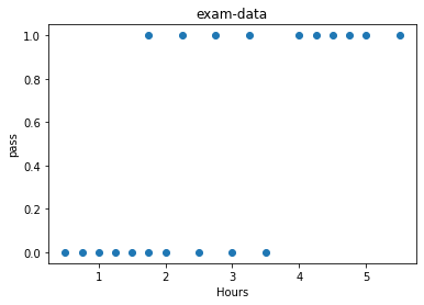
x=np.array([0.50,0.75,1.00,1.25,1.50,1.75,1.75,2.00,2.25,2.50,
2.75,3.00,3.25,3.50,4.00,4.25,4.50,4.75,5.00,5.50])
x=x.reshape(-1,1)
y=np.array([0,0,0,0,0,0,1,0,1,0,1,0,1,0,1,1,1,1,1,1])
x=np.concatenate((np.ones((x.shape[0],1)),x),axis=1)
y=y.reshape(-1,1)
y.shape
|
(20, 1)
1
2
3
4
5
| plt.scatter(x[:,1],y)
plt.xlabel('Hours')
plt.ylabel('pass')
plt.title('exam-data')
plt.show()
|
J(θ)=−m1i=1∑m(yilog(hθ(xi))+(1−yi)log(1−hθ(xi)))
θ∂J(θ)=m1∑i=1m(hθ(xi)−yi)xi
1
2
3
4
5
6
7
8
9
10
11
12
13
14
15
16
17
18
19
20
21
22
23
24
| def sigmoid(x):
return 1.0/(1+np.exp(-x))
def cost(x,y,theta):
x=np.matrix(x)
y=np.matrix(y)
theta=np.matrix(theta)
first=np.multiply(y,np.log(sigmoid(x*theta)))
second=np.multiply(1-y,np.log(1-sigmoid(x*theta)))
return np.sum(first+second)/(-len(x))
def grad(x,y,theta,epochs=1000,lr=0.001):
x=np.matrix(x)
y=np.matrix(y)
theta=np.matrix(theta)
m=x.shape[0]
costList=[]
for i in range(epochs+1):
h=sigmoid(x*theta)
delta=x.T*(h-y)/m
theta=theta-lr*delta
if(i%50==0):
costList.append(cost(x,y,theta))
return theta,costList
|
1
2
3
4
5
6
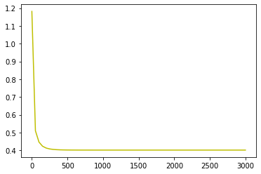
| theta=np.ones((x.shape[1],1))
theta,costList=grad(x,y,theta,3000,0.3)
a=np.linspace(0,3000,61)
plt.plot(a,costList,c='y')
plt.show()
|
1
2
3
4
5
6
7
8
9
10
11
12
| from sklearn.linear_model import LogisticRegression
x=np.array([0.50,0.75,1.00,1.25,1.50,1.75,1.75,2.00,2.25,2.50,
2.75,3.00,3.25,3.50,4.00,4.25,4.50,4.75,5.00,5.50])
x=x.reshape(-1,1)
y=np.array([0,0,0,0,0,0,1,0,1,0,1,0,1,0,1,1,1,1,1,1])
y=y.reshape(-1,1)
model=LogisticRegression()
model.fit(x,y)
b=model.intercept_
a=model.coef_
print(a,b)
print(theta)
|
[[1.14860386]] [-3.13952411]
[[-4.07770898]
 [ 1.50464392]]
1
2
3
4
5
6
7
8
9
10
| from sklearn.metrics import classification_report
def predect(x,theta):
x=np.matrix(x)
theta=np.matrix(theta)
return [1 if i>0.5 else 0 for i in (sigmoid(x*theta))]
x2=np.concatenate((np.ones((x.shape[0],1)),x),axis=1)
prediction=predect(x2,theta)
print(classification_report(y,prediction))
|
              precision    recall  f1-score   support

           0       0.80      0.80      0.80        10
           1       0.80      0.80      0.80        10

    accuracy                           0.80        20
   macro avg       0.80      0.80      0.80        20
weighted avg       0.80      0.80      0.80        20
可以看出正确率有80%
5.(补充)reshape函数
①numpy.arange(n).reshape(a, b) 依次生成n个自然数,并且以a行b列的数组形式显示
②mat (or array).reshape(c, -1) 必须是矩阵格式或者数组格式,才能使用 .reshape(c, -1) 函数, 表示将此矩阵或者数组重组,以 c行d列的形式表示
③reshape(1,-1)转化成1行
reshape(2,-1)转换成两行
reshape(-1,1)转换成1列
reshape(-1,2)转化成两列
>>> import numpy as np
>>> np.arange(16).reshape(2,8)#生成16个数,以2行8列形式显示
array([[ 0,  1,  2,  3,  4,  5,  6,  7],
       [ 8,  9, 10, 11, 12, 13, 14, 15]])
>>> a=np.arange(16).reshape(2,8)#生成16个数,以2行8列形式显示
>>> a.shape
(2, 8)
>>> a.reshape(4,-1)#改变为m行,d列(-1表示列数自动计算,d=a*b/m)
array([[ 0,  1,  2,  3],
       [ 4,  5,  6,  7],
       [ 8,  9, 10, 11],
       [12, 13, 14, 15]])
>>> a.reshape(-1,2)#改变为d行,m列(-1表示行数自动计算,d=a*b/m)
array([[ 0,  1],
       [ 2,  3],
       [ 4,  5],
       [ 6,  7],
       [ 8,  9],
       [10, 11],
       [12, 13],
       [14, 15]])
>>> np.array(1,12,2)#(a,b.c) 从数字a起,步长为c,到b结束
>>> np.arange(1,12,2)#(a,b.c) 从数字a起数,步长为c,到b结束
array([ 1,  3,  5,  7,  9, 11])
>>> a.reshape(1,-1)#1行
array([[ 0,  1,  2,  3,  4,  5,  6,  7,  8,  9, 10, 11, 12, 13, 14, 15]])
>>> a.reshape(2,-1)#2行
array([[ 0,  1,  2,  3,  4,  5,  6,  7],
       [ 8,  9, 10, 11, 12, 13, 14, 15]])
>>> a.reshape(-1,1)#一列
array([[ 0],
       [ 1],
       [ 2],
       [ 3],
       [ 4],
       [ 5],
       [ 6],
       [ 7],
       [ 8],
       [ 9],
       [10],
       [11],
       [12],
       [13],
       [14],
       [15]])
>>> a.reshape(-1,2)#2列
array([[ 0,  1],
       [ 2,  3],
       [ 4,  5],
       [ 6,  7],
       [ 8,  9],
       [10, 11],
       [12, 13],
       [14, 15]])
>>>